Machine Learning Notes: Vision Transformer (ViT)
(Please refer to Wow It Fits! — Secondhand Machine Learning. There are a lot of pictures in this post so it might take a while to load.)
Original paper is [2010.11929] An Image is Worth 16x16 Words: Transformers for Image Recognition at Scale. Here’s some notes from 08. PyTorch Paper Replicating - Zero to Mastery Learn PyTorch for Deep Learning.
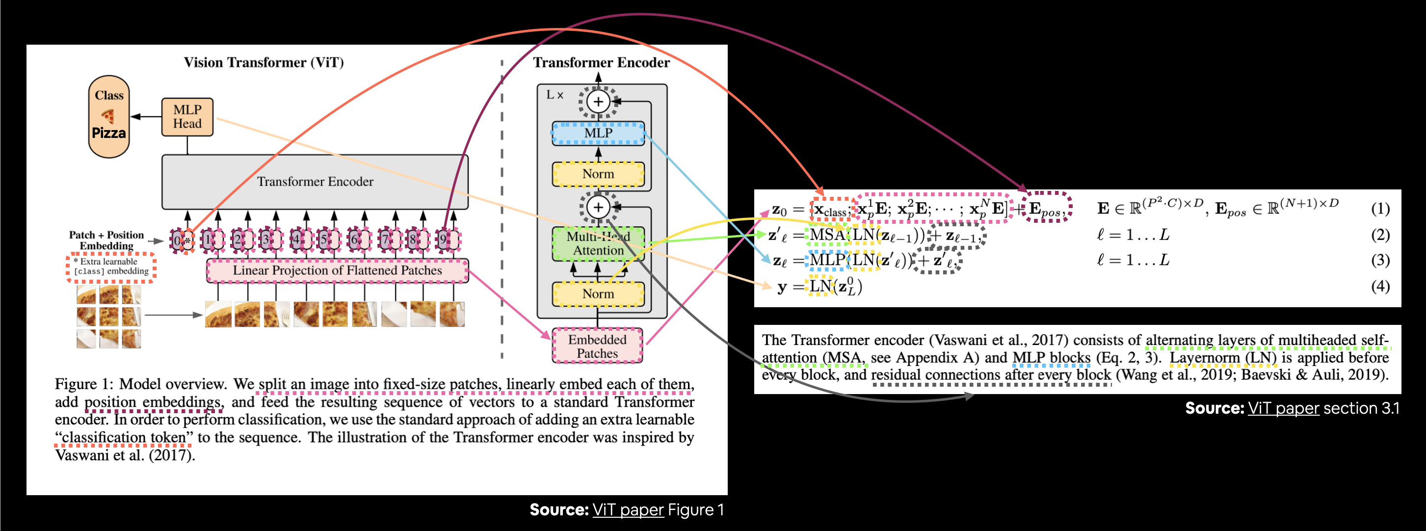
The relation between this structure and the equations:
First import packages:
import torch
import torch.nn as nn
import torch.nn.functional as F

from torchinfo import summary
§1 Embedding
This section is based on Eq. 1.
§1.1 Patch Embedding
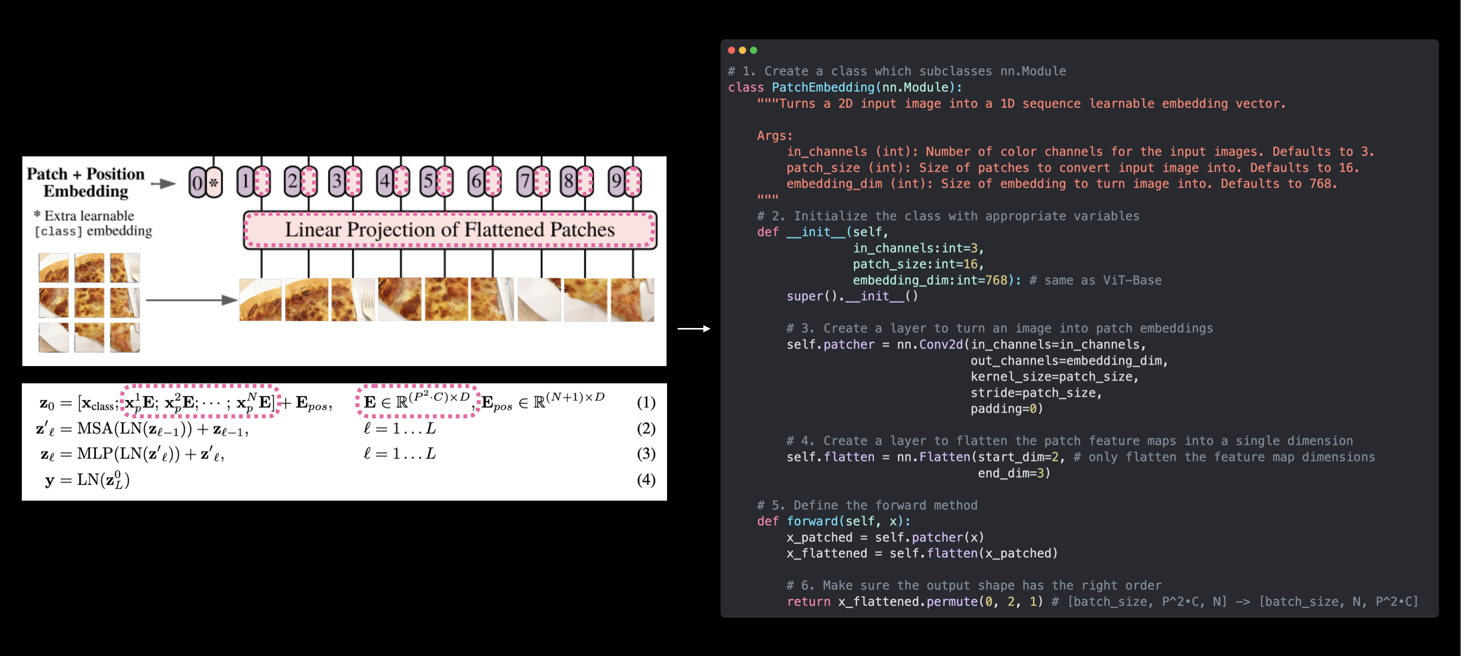
For $\mathbf{x} \in \mathbb{R}^{H \times W \times C} \rightarrow \mathbf{x}_{p} \in \mathbb{R}^{N \times\left(P^{2} \cdot C\right)}$, where $H$ is the height of the image, $W$ is the width of the image, $C$ is the color channel of the image (in this case the image is RGB, thus $C=3$), number of patches $N=H W / P^{2}$:
# 1. Create a class which subclasses nn.Module
class PatchEmbedding(nn.Module):
    """Turns a 2D input image into a 1D sequence learnable embedding vector.

    Args:
        in_channels (int): Number of color channels for the input images. Defaults to 3.
        patch_size (int): Size of patches to convert input image into. Defaults to 16.
        embedding_dim (int): Size of embedding to turn image into. Defaults to 768.
    """
    # 2. Initialize the class with appropriate variables
    def __init__(self,
                 in_channels:int=3,
                 patch_size:int=16,
                 embedding_dim:int=768):
        super().__init__()

        # 3. Create a layer to turn an image into patches
        self.patcher = nn.Conv2d(in_channels=in_channels,
                                 out_channels=embedding_dim,
                                 kernel_size=patch_size,
                                 stride=patch_size,# which means stride = kernel_size
                                 padding=0)

        # 4. Create a layer to flatten the patch feature maps into a single dimension
        self.flatten = nn.Flatten(start_dim=2, # only flatten the feature map dimensions into a single vector
                                  end_dim=3)

    # 5. Define the forward method
    def forward(self, x):
        # Create assertion to check that inputs are the correct shape
        # image_resolution = x.shape[-1]
        # assert image_resolution % patch_size == 0, f"Input image size must be divisble by patch size, image shape: {image_resolution}, patch size: {patch_size}"

        # Perform the forward pass
        x_patched = self.patcher(x)
        x_flattened = self.flatten(x_patched)
        # 6. Make sure the output shape has the right order
        return x_flattened.permute(0, 2, 1) # adjust so the embedding is on the final dimension [batch_size, P^2•C, N] -> [batch_size, N, P^2•C]
To use PatchEmbedding:
dummy = torch.rand(1, 3, 224, 224)
print(f"Input image with batch dimension shape: {dummy.shape}")# [batch_size, C, W, H]

# Create an instance of class PatchEmbedding
patchify = PatchEmbedding(in_channels=3, patch_size=16, embedding_dim=768)
print(f"Patching embedding shape: {patchify(dummy).shape}")# [batch_size, N, P^2•C]
will get:
Input image with batch dimension shape: torch.Size([1, 3, 224, 224])
Patching embedding shape: torch.Size([1, 196, 768])
§1.2 Class Token Embedding, Position Embedding and Put them together
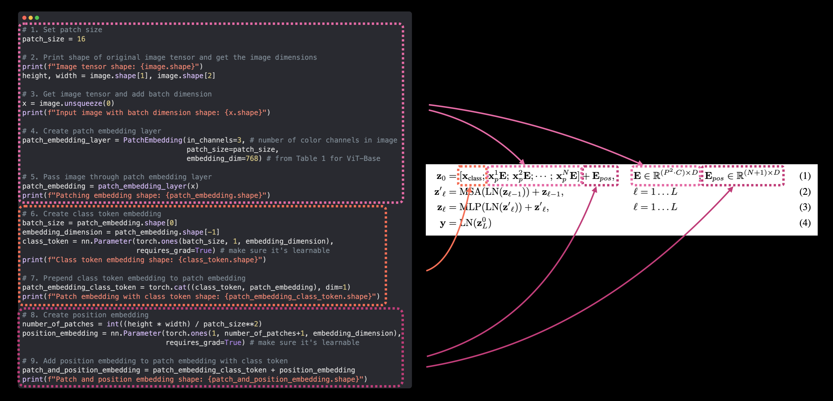
image = torch.rand(3, 224, 224)

# 1. Set patch size
patch_size = 16

# 2. Print shape of original image tensor and get the image dimensions
print(f"Image tensor shape: {image.shape}")
height, width = image.shape[1], image.shape[2]

# 3. Get image tensor and add batch dimension
x = image.unsqueeze(0)
print(f"Input image with batch dimension shape: {x.shape}")

# 4. Create patch embedding layer
patch_embedding_layer = PatchEmbedding(in_channels=3,
                                       patch_size=16,
                                       embedding_dim=768)

# 5. Pass image through patch embedding layer
patch_embedding = patch_embedding_layer(x)
print(f"Patching embedding shape: {patch_embedding.shape}")

# 6. Create class token embedding
batch_size = patch_embedding.shape[0]
embedding_dimension = patch_embedding.shape[-1]
class_token = nn.Parameter(torch.ones(batch_size, 1, embedding_dimension),
                           requires_grad=True) # make sure it's learnable
print(f"Class token embedding shape: {class_token.shape}")

# 7. Prepend class token embedding to patch embedding
patch_embedding_class_token = torch.cat((class_token, patch_embedding), dim=1)
print(f"Patch embedding with class token shape: {patch_embedding_class_token.shape}")

# 8. Create position embedding
number_of_patches = int((height * width) / patch_size**2)
position_embedding = nn.Parameter(torch.ones(1, number_of_patches+1, embedding_dimension),
                                  requires_grad=True) # make sure it's learnable
print(f"Position embedding shape: {position_embedding.shape}")

# 9. Add position embedding to patch embedding with class token
patch_and_position_embedding = patch_embedding_class_token + position_embedding
print(f"Patch and position embedding shape: {patch_and_position_embedding.shape}")
will get:
Image tensor shape: torch.Size([3, 224, 224])
Input image with batch dimension shape: torch.Size([1, 3, 224, 224])
Patching embedding shape: torch.Size([1, 196, 768])
Class token embedding shape: torch.Size([1, 1, 768])
Patch embedding with class token shape: torch.Size([1, 197, 768])
Position embedding shape: torch.Size([1, 197, 768])
Patch and position embedding shape: torch.Size([1, 197, 768])
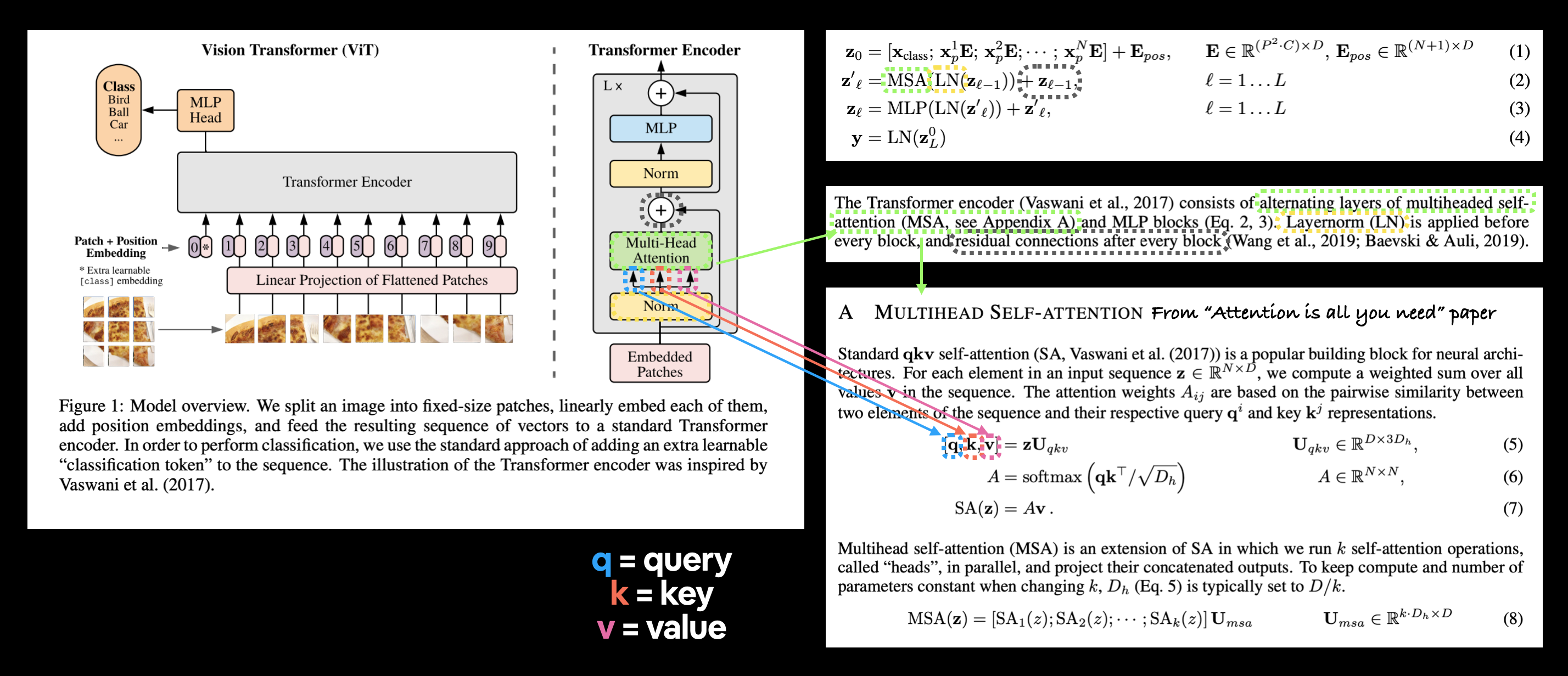
§2 Multi-Head Self Attention (MSA)
This section is based on Eq. 2.
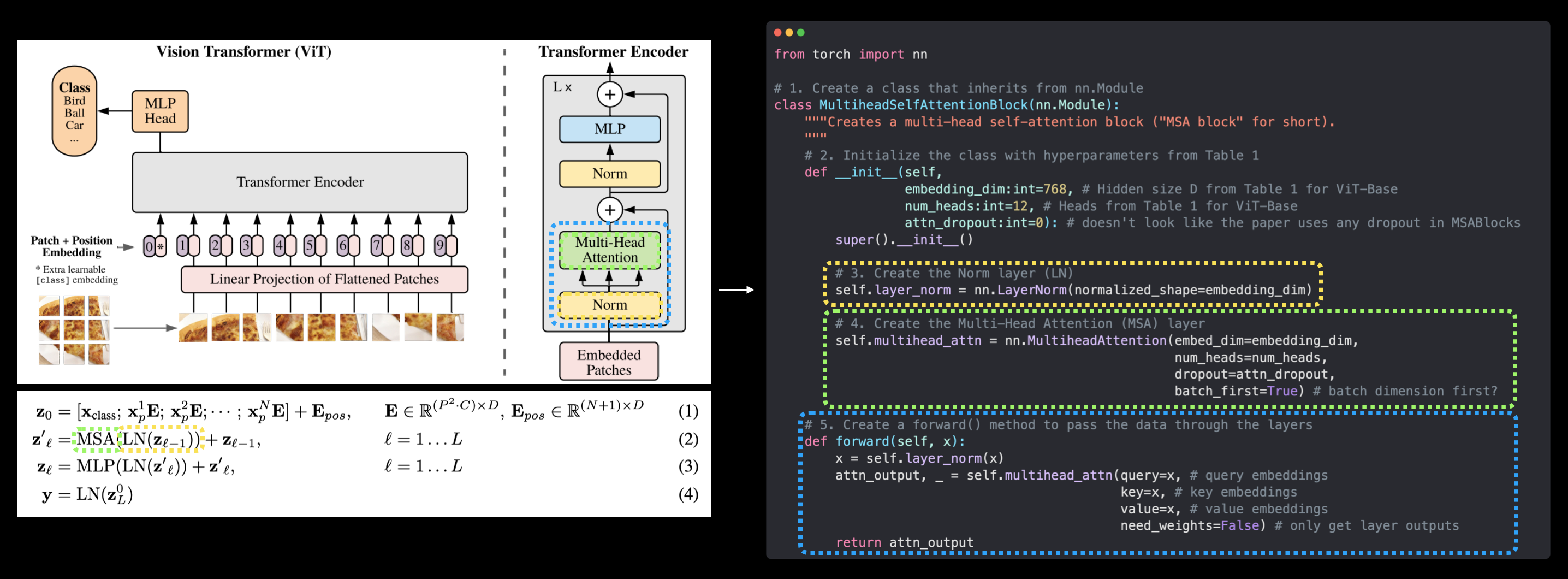
# 1. Create a class that inherits from nn.Module
class MultiheadSelfAttentionBlock(nn.Module):
    """Creates a multi-head self-attention block ("MSA block" for short).
    """
    # 2. Initialize the class with hyperparameters from Table 1
    def __init__(self,
                 embedding_dim:int=768, # Hidden size D from Table 1 for ViT-Base
                 num_heads:int=12, # Heads from Table 1 for ViT-Base
                 attn_dropout:float=0): # doesn't look like the paper uses any dropout in MSABlocks
        super().__init__()

        # 3. Create the Norm layer (LN)
        self.layer_norm = nn.LayerNorm(normalized_shape=embedding_dim)

        # 4. Create the Multi-Head Attention (MSA) layer
        self.multihead_attn = nn.MultiheadAttention(embed_dim=embedding_dim,
                                                    num_heads=num_heads,
                                                    dropout=attn_dropout,
                                                    batch_first=True) # does our batch dimension come first?

    # 5. Create a forward() method to pass the data throguh the layers
    def forward(self, x):
        x = self.layer_norm(x)
        attn_output, _ = self.multihead_attn(query=x, # query embeddings
                                             key=x, # key embeddings
                                             value=x, # value embeddings
                                             need_weights=False) # do we need the weights or just the layer outputs?
        return attn_output
To use MultiheadSelfAttentionBlock:
# Create an instance of MSABlock, embedding_dim and num_heads are from Table 1
multihead_self_attention_block = MultiheadSelfAttentionBlock(embedding_dim=768,
                                                             num_heads=12)

# Pass patch and position image embedding through MSABlock
patched_image_through_msa_block = multihead_self_attention_block(patch_and_position_embedding)
# or
# patched_image_through_msa_block = multihead_self_attention_block(torch.rand(1, 197, 768))
print(f"Input shape of MSA block: {patch_and_position_embedding.shape}")
print(f"Output shape MSA block: {patched_image_through_msa_block.shape}")
will get:
Input shape of MSA block: torch.Size([1, 197, 768])
Output shape MSA block: torch.Size([1, 197, 768])
Note that input and output have the same shape, which is common for different kinds of AttentionBlock.
§3 Multilayer Perception (MLP)
This section is based on Eq. 3.

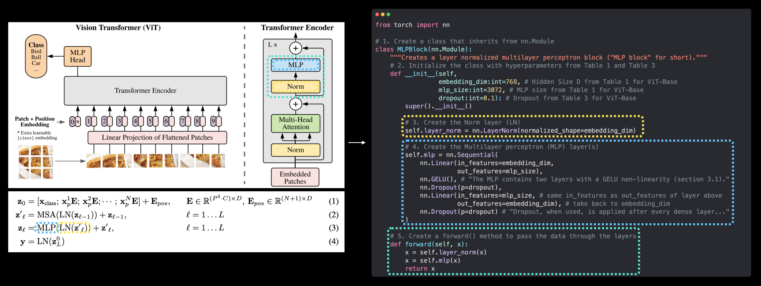
# 1. Create a class that inherits from nn.Module
class MLPBlock(nn.Module):
    """Creates a layer normalized multilayer perceptron block ("MLP block" for short)."""
    # 2. Initialize the class with hyperparameters from Table 1 and Table 3
    def __init__(self,
                 embedding_dim:int=768, # Hidden Size D from Table 1 for ViT-Base
                 mlp_size:int=3072, # MLP size from Table 1 for ViT-Base
                 dropout:float=0.1): # Dropout from Table 3 for ViT-Base
        super().__init__()

        # 3. Create the Norm layer (LN)
        self.layer_norm = nn.LayerNorm(normalized_shape=embedding_dim)

        # 4. Create the Multilayer perceptron (MLP) layer(s)
        self.mlp = nn.Sequential(
            nn.Linear(in_features=embedding_dim,
                      out_features=mlp_size),
            nn.GELU(), # "The MLP contains two layers with a GELU non-linearity (section 3.1)."
            nn.Dropout(p=dropout),
            nn.Linear(in_features=mlp_size, # needs to take same in_features as out_features of layer above
                      out_features=embedding_dim), # take back to embedding_dim
            nn.Dropout(p=dropout) # "Dropout, when used, is applied after every dense layer.."
        )

    # 5. Create a forward() method to pass the data throguh the layers
    def forward(self, x):
        x = self.layer_norm(x)
        x = self.mlp(x)
        return x
To use MLPBlock:
# Create an instance of MLPBlock
mlp_block = MLPBlock(embedding_dim=768, # from Table 1
                     mlp_size=3072, # from Table 1
                     dropout=0.1) # from Table 3

# Pass output of MSABlock through MLPBlock
patched_image_through_mlp_block = mlp_block(patched_image_through_msa_block)
# or
# patched_image_through_msa_block = mlp_block(torch.rand(1, 197, 768))
print(f"Input shape of MLP block: {patched_image_through_mlp_block.shape}")
print(f"Output shape MLP block: {patched_image_through_mlp_block.shape}")
will get:
Input shape of MLP block: torch.Size([1, 197, 768])
Output shape MLP block: torch.Size([1, 197, 768])
Note that, again, input and output have the same shape.
§4 Transformer Encoder


§4.1 Put Blocks Above Together
# 1. Create a class that inherits from nn.Module
class TransformerEncoderBlock(nn.Module):
    """Creates a Transformer Encoder block."""
    # 2. Initialize the class with hyperparameters from Table 1 and Table 3
    def __init__(self,
                 embedding_dim:int=768, # Hidden size D from Table 1 for ViT-Base
                 num_heads:int=12, # Heads from Table 1 for ViT-Base
                 mlp_size:int=3072, # MLP size from Table 1 for ViT-Base
                 mlp_dropout:float=0.1, # Amount of dropout for dense layers from Table 3 for ViT-Base
                 attn_dropout:float=0): # Amount of dropout for attention layers
        super().__init__()

        # 3. Create MSA block (equation 2)
        self.msa_block = MultiheadSelfAttentionBlock(embedding_dim=embedding_dim,
                                                     num_heads=num_heads,
                                                     attn_dropout=attn_dropout)

        # 4. Create MLP block (equation 3)
        self.mlp_block =  MLPBlock(embedding_dim=embedding_dim,
                                   mlp_size=mlp_size,
                                   dropout=mlp_dropout)

    # 5. Create a forward() method
    def forward(self, x):

        # 6. Create residual connection for MSA block (add the input to the output)
        x =  self.msa_block(x) + x

        # 7. Create residual connection for MLP block (add the input to the output)
        x = self.mlp_block(x) + x

        return x
Use torchinfo.summary to get the information about transformer_encoder_block:
# Create an instance of TransformerEncoderBlock
transformer_encoder_block = TransformerEncoderBlock()

# Print an input and output summary of our Transformer Encoder (uncomment for full output)
summary(model=transformer_encoder_block,
        input_size=(1, 197, 768), # (batch_size, num_patches, embedding_dimension)
        col_names=["input_size", "output_size", "num_params"],
        col_width=20,
        row_settings=["var_names"])
will get:

§4.2 Build Encoder with torch.nn.TransformerEncoderLayer():
# Create the same as above with torch.nn.TransformerEncoderLayer()
torch_transformer_encoder_layer = nn.TransformerEncoderLayer(d_model=768, # Hidden size D from Table 1 for ViT-Base
                                                             nhead=12, # Heads from Table 1 for ViT-Base
                                                             dim_feedforward=3072, # MLP size from Table 1 for ViT-Base
                                                             dropout=0.1, # Amount of dropout for dense layers from Table 3 for ViT-Base
                                                             activation="gelu", # GELU non-linear activation
                                                             batch_first=True, # Do our batches come first?
                                                             norm_first=True) # Normalize first or after MSA/MLP layers?
Use torchinfo.summary to get the information about torch_transformer_encoder_layer:
# Get the output of PyTorch's version of the Transformer Encoder (uncomment for full output)
summary(model=torch_transformer_encoder_layer,
        input_size=(1, 197, 768), # (batch_size, num_patches, embedding_dimension)
        col_names=["input_size", "output_size", "num_params", "trainable"],
        col_width=10,
        row_settings=["var_names"])
will get:

Using torch.nn will be slightly different, they have $\mathrm{3}$ advantages in general:
- Faster.
- More robust.
- Easier to build.
§5 ViT
Eq. 4 is the final torch.nn.LayerNorm() and torch.nn.Linear.
# 1. Create a ViT class that inherits from nn.Module
class ViT(nn.Module):
    """Creates a Vision Transformer architecture with ViT-Base hyperparameters by default."""
    # 2. Initialize the class with hyperparameters from Table 1 and Table 3
    def __init__(self,
                 img_size:int=224, # Training resolution from Table 3 in ViT paper
                 in_channels:int=3, # Number of channels in input image
                 patch_size:int=16, # Patch size
                 num_transformer_layers:int=12, # Layers from Table 1 for ViT-Base
                 embedding_dim:int=768, # Hidden size D from Table 1 for ViT-Base
                 mlp_size:int=3072, # MLP size from Table 1 for ViT-Base
                 num_heads:int=12, # Heads from Table 1 for ViT-Base
                 attn_dropout:float=0, # Dropout for attention projection
                 mlp_dropout:float=0.1, # Dropout for dense/MLP layers
                 embedding_dropout:float=0.1, # Dropout for patch and position embeddings
                 num_classes:int=1000): # Default for ImageNet but can customize this
        super().__init__() # don't forget the super().__init__()!

        # 3. Make the image size is divisble by the patch size
        assert img_size % patch_size == 0, f"Image size must be divisible by patch size, image size: {img_size}, patch size: {patch_size}."

        # 4. Calculate number of patches (height * width/patch^2)
        self.num_patches = (img_size * img_size) // patch_size**2

        # 5. Create learnable class embedding (needs to go at front of sequence of patch embeddings)
        self.class_embedding = nn.Parameter(data=torch.randn(1, 1, embedding_dim),
                                            requires_grad=True)

        # 6. Create learnable position embedding
        self.position_embedding = nn.Parameter(data=torch.randn(1, self.num_patches+1, embedding_dim),
                                               requires_grad=True)

        # 7. Create embedding dropout value
        self.embedding_dropout = nn.Dropout(p=embedding_dropout)

        # 8. Create patch embedding layer
        self.patch_embedding = PatchEmbedding(in_channels=in_channels,
                                              patch_size=patch_size,
                                              embedding_dim=embedding_dim)

        # 9. Create Transformer Encoder blocks (we can stack Transformer Encoder blocks using nn.Sequential())
        # Note: The "*" means "all"
        self.transformer_encoder = nn.Sequential(*[TransformerEncoderBlock(embedding_dim=embedding_dim,
                                                                            num_heads=num_heads,
                                                                            mlp_size=mlp_size,
                                                                            mlp_dropout=mlp_dropout) for _ in range(num_transformer_layers)])

        # 10. Create classifier head
        self.classifier = nn.Sequential(
            nn.LayerNorm(normalized_shape=embedding_dim),
            nn.Linear(in_features=embedding_dim,
                      out_features=num_classes)
        )

    # 11. Create a forward() method
    def forward(self, x):

        # 12. Get batch size
        batch_size = x.shape[0]

        # 13. Create class token embedding and expand it to match the batch size (equation 1)
        class_token = self.class_embedding.expand(batch_size, -1, -1) # "-1" means to infer the dimension (try this line on its own)

        # 14. Create patch embedding (equation 1)
        x = self.patch_embedding(x)

        # 15. Concat class embedding and patch embedding (equation 1)
        x = torch.cat((class_token, x), dim=1)

        # 16. Add position embedding to patch embedding (equation 1)
        x = self.position_embedding + x

        # 17. Run embedding dropout (Appendix B.1)
        x = self.embedding_dropout(x)

        # 18. Pass patch, position and class embedding through transformer encoder layers (equations 2 & 3)
        x = self.transformer_encoder(x)

        # 19. Put 0 index logit through classifier (equation 4)
        x = self.classifier(x[:, 0]) # run on each sample in a batch at 0 index

        return x
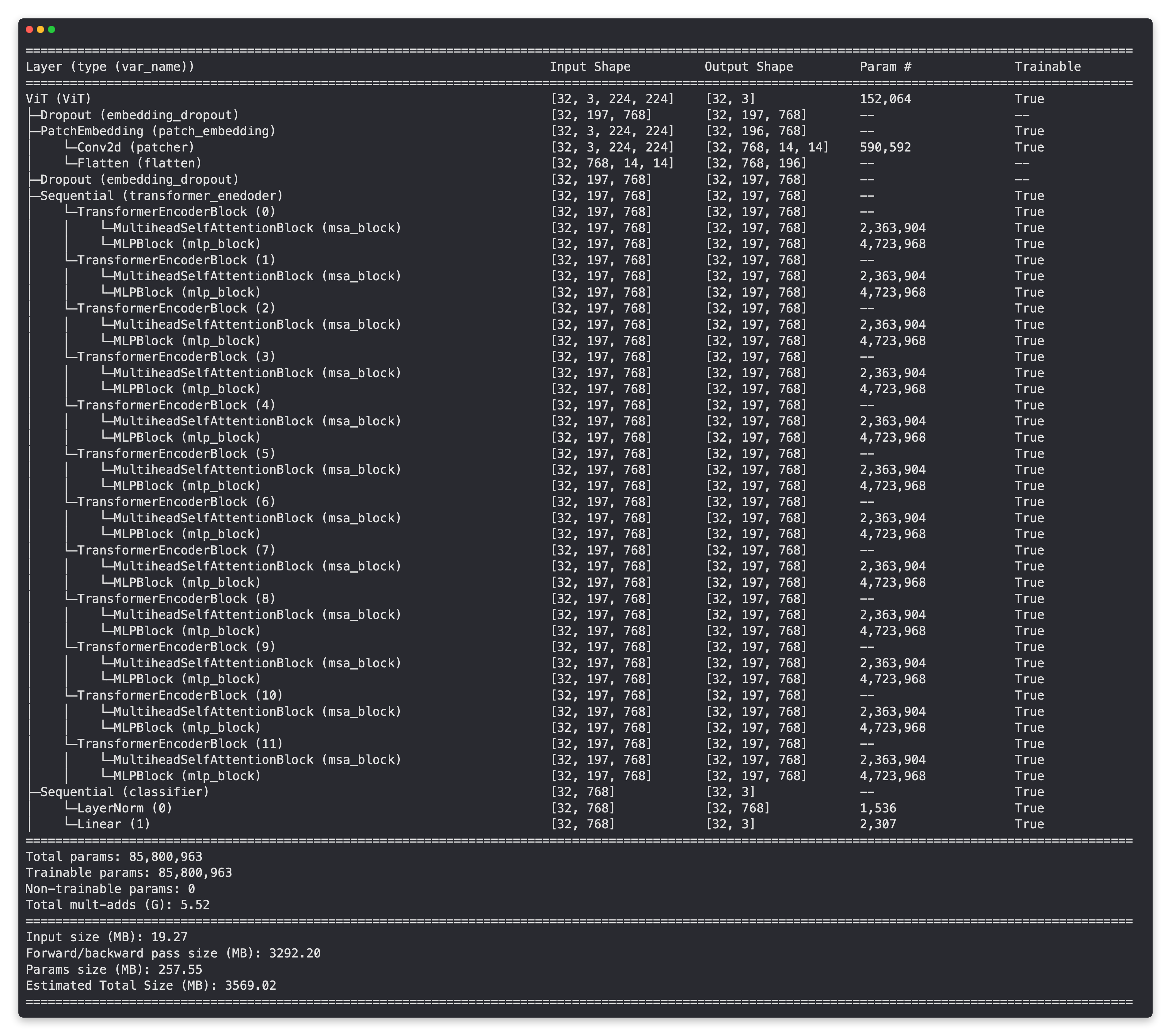
Use torchinfo.summary to get the information about torch_transformer_encoder_layer:
# Create a random tensor with same shape as a single image
random_image_tensor = torch.randn(1, 3, 224, 224) # (batch_size, color_channels, height, width)

# Create an instance of ViT with the number of classes we're working with (pizza, steak, sushi)
# vit = ViT(num_classes=len(class_names))
vit = ViT(num_classes=3)

# Print a summary of our custom ViT model using torchinfo (uncomment for actual output)
summary(model=vit,
        input_size=(32, 3, 224, 224), # (batch_size, color_channels, height, width)
        # col_names=["input_size"], # uncomment for smaller output
        col_names=["input_size", "output_size", "num_params", "trainable"],
        col_width=20,
        row_settings=["var_names"]
)
will get:
§6 Optimizer, Loss Function
Generally these two will be different in different model, I’ll write about them later.
In ViT they are torch.optim.Adam() and torch.nn.CrossEntropyLoss(), see Section 9. Setting up training code for our ViT model.
§7 Use Pretrained model (Transfer Learning)
See Section 10. Using a pretrained ViT from torchvision.models on the same dataset.
For more information on Transfer Learning, see 06. PyTorch Transfer Learning. Freeze part of the model and train the rest of the model is fun. I will get to this some day, but since in physics we are dealing with quite different dataset than Natural Language Processing (NLP) or Computer Vision (CV), it’s probably not gonna be really helpful. Except classification for Galaxies or Gravitational Wave, which are close to traditional CV classification missions.
§8 CNN or Transformer
The comparison of CNN and Transformer in Section 10.6 Save feature extractor ViT model and check file size is interesting.
But transformer is better than CNN in $\mathrm{2}$ ways:
- Multimodal. Embedding then
torch.catis surprisingly useful. - No signs of overfitting yet.
At scale, they tend to have same performance, see [2310.16764] ConvNets Match Vision Transformers at Scale.